21. A tutorial on Markov Chain Monte Carlo¶

References for today’s lecture:

Davidson-Pilon, “Bayesian methods for hackers”, Addison Wesley, 2016, Chapter 2 and 3
Jan-Willem van de Meent et al. “An Introduction to Probabilistic Programming”

21.1. The Bayesian setting¶

In the frequentist approach to inference the probability of an event is defined in terms of its propensity to ocurr (how frequent it ocurrs). In contrast, bayesians interpret probability as our knowledge (or lack of knowledge) of the event. Probability quantifies the uncertainty of the event.

We will use a random variable \(\theta\) to represent this event. Our current belief of this event is \(p(\theta)\), the prior probability distribution.

Then we collect data \(\mathcal{D}\) and update our belief about \(\theta\) by forming a posterior distribution \(p(\theta|\mathcal{D})\)

Obtaining the posterior from the prior and the data is done using Bayes Theorem:

\[ p(\theta|\mathcal{D}) = \frac{p(\mathcal{D}|\theta)p(\theta)}{p(X)} = \frac{p(\mathcal{D}|\theta)p(\theta)}{\int p(\mathcal{D}, \theta) \, d\theta} = \frac{p(\mathcal{D}|\theta)p(\theta)}{\int p(\mathcal{D}|A\theta)p(\theta) \,d\theta}, \]

where we also used the law of total probability to write the marginal likelihood \(p(\mathcal{D})\) in terms of the likelihood and the prior.

Only for a few models (conjugate priors) this expresion is tractable. The intractability comes from the integral in the denominator.

To obtain the posterior for more complex models we resort to approximate inference technices or Monte-Carlo Markov Chain (MCMC). We will review the latter in this lesson.

21.2. Monte Carlo Integration¶

Monte carlo methods obtain numerical results via repeated random sampling. One of its most important case uses is Monte-carlo integration.

Let’s say we want the expected value of a function \(g\) over a random variable \(X\) with distribution \(f(x)\), by definition this is

\[ \mathbb{E}[g(X)] = \int g(x) f(x) \,dx \]

If this integral is hard to compute and we have samples from \(f(x)\) then we can approximate the expected value using Monte Carlo integration

\[ \mathbb{E}[g(X)] \approx \hat g_N = \frac{1}{N} \sum_{i=1}^N g(x_i) \quad x_i \sim f(x) \]

and due to the Central Limit Theorem we have that

\[ \hat g_N \sim \mathcal{N} \left( \mathbb{E}[g(X)], \sigma_N^2/N \right) \]

i.e. the more samples we use the more concentrated on the real value our estimate is

21.3. From Monte Carlo to Markov Chain Monte Carlo¶

The problem with Monte Carlo integration is that in some cases we can’t draw samples from distribution \(f\). Also randomly sampling in all the space of \(f\) is very inefficient

To obtain samples from distributions that we can only evaluate up to their normalizing constant, such as the posterior \(p(\theta|\mathcal{D})\) we can use Markov Chain Monte Carlo (MCMC)

MCMC is a family of algorithms that learn the transition probabilities of a markov chain so that it converges to a desired distribution. A Markov Chain is a random process \(\{X_n\}_{n=0,1,\ldots}\), i.e. a sequence of random variables, with the following property

\[ p(X_n|X_{n-1},\ldots, X_0) = p(X_n|X_{n-1}) \]

Importante

In a Markov chain the probability of the future is conditionally independant of the past given the present

Markov chains that are irreducible converge in the long term to a stationary distribution. MCMC methods are based on the idea of building a Markov Chain so that it converges to the distribution we are interested in, e.g. a bayesian posterior

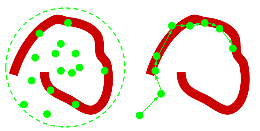
In the following diagram, we want samples from the red distribution. The diagram on the left uses importance sampling. The diagram on the right uses MCMC

MCMC searches the space in a less naive way. The sequence of samples from the Markov Chain is called a trace

The key in MCMC methods lays in how we choose the transition probability of the chain, i.e. how do we choose the next point in the chain. There are several “proposal” algorithms, two of the most popular ones being

Metropolis Hastings (MH)

Random walker that moves on all dimensions simultaneously
A candidate step is drawn from an arbitrary but symmetric distribution \(x^{new} \sim g(x^{new}|x_t)\)
We accept the step if \(f(x^{new})/f(x^t)\) is equal or larger than a certain threshold. Note that \(f(\cdot)\) needs only to be proportional to the target distribution (evidence is canceled in the ratio)
Repeat many times until convergence

Hamiltonian Monte-Carlo

Family of step proposing methods that use momentum (derivatives). Only for continuous variables
Costs more than MH (single iteration) but require less iterations
http://arogozhnikov.github.io/2016/12/19/markov_chain_monte_carlo.html

21.4. Probabilistic programming (PP)¶

Excerpt from https://probabilistic-programming.org/:

Probabilistic programming languages aim to unify general purpose programming with probabilistic modeling. The user specifies the probabilistic model (priors, likelihood, etc) and inference follows automatically given the specification

Python friendly PP frameworks/libraries:

PyMC3: Black-box VI, MH, Gibbs, NUTS sampler. Uses theano
PyStan: Python interface for Stan platform
emcee: Pure python implementation of the Affine invariant MCMC ensemble sampler
Edward: Black-box VI, neural networks. Uses tensorflow
Pyro: Black-box VI, neural networks, MCMC. Uses pytorch
NumPyro: Black-box VI and MCMC. Uses JAX

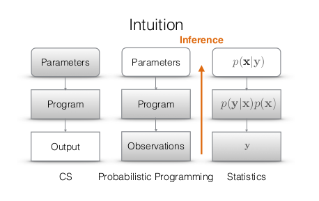
The following is a diagram contrasting traditional programming with PP

PP runs in two directions!

21.5. A `numpyro` tutorial (bayesian logistic regression)¶

In this tutorial we will review how to do

Define a model
Obtain a trace using MCMC
Assess the convergence of the chain
Use the posterior to do predictive inference

with the numpyro library

We will do this through an example: Bayesian logistic regression

true_coef = [-0.5, -1, 2]
N = 30
x = dist.Normal(0, 1).sample(random.PRNGKey(1), sample_shape=(N, 2))
y = dist.Bernoulli(logits=true_coef[0] + true_coef[1]*x[:, 0] + true_coef[2]*x[:, 1]).sample(random.PRNGKey(1))

p1 = hv.Scatter((x[y==0, 0], x[y==0, 1]), kdims=['x[:, 1]'], vdims=['x[:, 0]'], label='y==0').opts(size=10, marker='d')
p2 = hv.Scatter((x[y==1, 0], x[y==1, 1]), label='y==1').opts(size=10, marker='o')
hv.Overlay([p1, p2]).opts(legend_position='top')

21.5.1. Model specification¶

For this model we will assume:

Two deterministic independent variables
Gaussian priors with zero mean and standard deviation equal to 10 for the regression coefficients \(\theta\)
Three parameters: intercept plus one parameter per independent variable
Response (dependent variable) is binary. Likelihood with Bernoulli distribution

Mathematically, the relation between the independent variable \(X\) and the dependent variable \(Y\) is

\[ y = \text{sigmoid}(\theta_0 + \theta_1 x_1 + \theta_2 x_2) \]

where

\[ \text{sigmoid}(z) = \frac{1}{1 + e^{-z}} \]

In numpyro a model is defined as a function. We use the following primitives

numpyro.sample to declare random variables. Expects a name and a distribution.
numpyro.deterministic to declare deterministic variables that we want to track. Expects a name and a value
numpyro.plate to declare conditional independence on our data. Expects a name and a size

The bayesian regression model is then

import numpyro.distributions as dist

def sigmoid(z):
    return 1/(1 + jnp.exp(-z))

def model(x, y=None):
    theta_dist = dist.Normal(loc=jnp.zeros(3), scale=5*jnp.ones(3)).to_event(1)
    theta = numpyro.sample("theta", theta_dist)    
    with numpyro.plate('data', size=len(x)):
        logitp = theta[0] + x[:, 0]*theta[1] + x[:, 1]*theta[2]
        p = sigmoid(numpyro.deterministic('p', value=logitp))
        numpyro.sample("y", dist.Bernoulli(probs=p), obs=y)
        return p

Note that

priors are random variables with no observed data
the likelihood is given the data (dependent variable) through the obs keyword argument

We can check if the dimensions of the variables are correct using numpyro.handlers

seeded_model = numpyro.handlers.seed(model, random.PRNGKey(1234))
exec_trace = numpyro.handlers.trace(seeded_model).get_trace(x, y)
print(numpyro.util.format_shapes(exec_trace))

Trace Shapes:       
 Param Sites:       
Sample Sites:       
   theta dist    | 3
        value    | 3
   data plate 30 |  
       y dist 30 |  
        value 30 |  

We can use the seed handler to sample from the model

for i in range(3): # Three arbitrary seeds
    seeded_model = numpyro.handlers.seed(model, random.PRNGKey(i))
    print(i, seeded_model(x))

[0.9483369  0.9961683  0.9986565  0.99999905 0.948488   0.8254224
99699914 0.9940858  0.66100204 0.99964213 0.9999877  0.9999981
6035196  0.9389754  0.9999969  0.7939723  0.99830925 0.936527
9999622  0.9146049  0.00174457 0.7273527  0.18515117 0.04904454
91679025 0.99965346 0.99999905 0.9851034  0.06928106 0.99830014]
[9.8193890e-01 3.3314258e-01 1.5257716e-01 7.0865053e-06 9.3212968e-01
9969864e-01 9.9437040e-01 3.7644054e-03 9.9999917e-01 9.8115957e-01
7127444e-01 2.3044339e-07 9.9999976e-01 9.9999630e-01 9.7828195e-04
7756959e-01 1.3032483e-01 9.9954849e-01 5.4665125e-04 9.9998569e-01
0000000e+00 9.9996567e-01 9.9999976e-01 1.0000000e+00 9.9999619e-01
7421265e-01 6.7606627e-05 2.8816512e-01 9.9997127e-01 6.7209448e-03]
[7.5644083e-02 1.2386155e-01 9.4867848e-02 8.5689329e-02 1.5991542e-01
1121141e-02 3.0641246e-03 8.0771714e-01 1.2049341e-03 9.9392806e-04
6270703e-05 5.7761908e-01 8.2400028e-04 5.1014172e-04 1.2192503e-02
3741547e-01 1.2572035e-01 1.0032027e-02 1.3701907e-01 1.6046116e-03
1400842e-03 9.2949448e-03 3.5460973e-03 1.1311474e-03 6.9401605e-04
1769410e-03 2.2065228e-02 3.5016519e-01 1.6551776e-01 4.9304497e-01]

21.5.2. Obtaining posterior samples using MCMC¶

In numpyro MCMC is performed using

numpyro.infer.MCMC(sampler, # A sampler algorithms, e.g. NUTS, MH, Gibbs
                   num_warmup, # Number of initial samples to discard
                   num_samples, # Length of the trace (after discarding num_warmup samples)
                   num_chains=1, # Number of chains
                   ... 
                  )

which returns an object with the following methods

run(): Runs the sampler and fills the chain. It expects a random seed and the same arguments of the model function
print_summary(): Returns a table with the statistical moments of the parameters and some diagnostics
get_sample(): Returns the trace, i.e. the posterior samples

The sampler argument of MCMC expects an instance of MCMCKernel. Check the docs to see the samplers already implemented in numpyro.

In this case we will use the No-U Turn (NUTS) sampler, which is the state of the art for continuous parameters

rng_key = random.PRNGKey(12345)
rng_key, rng_key_ = random.split(rng_key)

sampler = numpyro.infer.MCMC(sampler=numpyro.infer.NUTS(model), 
                             num_samples=1000, num_warmup=100, thinning=1,
                             num_chains=2, progress_bar=False)

sampler.run(rng_key_, x, y)

/home/phuijse/.conda/envs/info320/lib/python3.9/site-packages/numpyro/infer/mcmc.py:274: UserWarning: There are not enough devices to run parallel chains: expected 2 but got 1. Chains will be drawn sequentially. If you are running MCMC in CPU, consider using `numpyro.set_host_device_count(2)` at the beginning of your program. You can double-check how many devices are available in your system using `jax.local_device_count()`.
  warnings.warn(

21.5.3. Convergence check¶

As mentioned we can do a “coarse” inspection using

sampler.print_summary()

                mean       std    median      5.0%     95.0%     n_eff     r_hat
  theta[0]     -0.36      0.54     -0.36     -1.20      0.54   1380.46      1.00
  theta[1]     -1.26      0.63     -1.21     -2.34     -0.31   1573.69      1.00
  theta[2]      1.42      0.61      1.39      0.42      2.38   1325.78      1.00

Number of divergences: 0

The Gelman Rubin statistics (\(\hat r\)) compares the variance between multiple chains to the variance within each chain. A value close to 1.0 means that all chains arrive to similar stationary distributions

The table also shows that

There were no divergences during sampling
The effective number of samples is more than 50%

All signs of a good convergence of the chain. We can also inspect the actual traces

posterior_samples = sampler.get_samples()
posterior_samples.keys()

dict_keys(['p', 'theta'])

traces = []
dists = []
for d in range(3):
    traces.append(hv.Curve((posterior_samples['theta'][:, d]), 
                           'Step', 'Theta', label=f'theta {d}').opts(alpha=0.75))
    dists.append(hv.Distribution(posterior_samples['theta'][:, d], 'Theta').opts(width=200))
hv.Overlay(traces).opts(legend_position='top') << hv.Overlay(dists)

If the markov chain reached its stationary distribution the traces should look like random noise around a certain value, which is the case here.

If the traces look like they are still going up or down, then you might need to sample longer. If the trace have sudden jumps (divergences) then the model might be mispecified

A more quantitative inspection of traces involves calculating their autocorrelation. The autocorrelation of a trace from a markov chain that have converged should go quickly to zero.

Now that we have confidence on our traces let’s do something useful with the posterior

21.5.4. Draw samples from the posterior predictive distribution¶

In practice, for a regressor, we want the posterior predictive distribution, i.e. the prediction y for a new sample x given the training dataset

\[ p(\textbf{y}|\textbf{x}, \mathcal{D}) = \int p(\textbf{y}|\textbf{x},\theta) p(\theta| \mathcal{D}) \,d\theta \]

where \(p(\theta| \mathcal{D})\) is the posterior of the parameters, and also the hardest term to obtain. Luckily we already have plenty of samples from this posterior

In NumPyro we can use

predictive = numpyro.infer.Predictive(model, posterior_samples=posterior_samples)

which returns an object that can be evaluated on new data

x_test = np.array([[-3, 1], 
                   [3, -1], 
                   [0.5, 0.5]])

posterior_predictive_samples = predictive(random.PRNGKey(1), x_test)
display(posterior_predictive_samples.keys(), 
        posterior_predictive_samples['y'].shape)

dict_keys(['p', 'y'])

(2000, 3)

Nota

Since our trace has 2000 samples we obtain 2000 values for the prediction of each data sample in x_test

We have obtained a distribution for the predictions. From this distribution we can obtain the most probable prediction and also the associated uncertainty.

for i, sample in enumerate(posterior_predictive_samples['y'].T):
    print(f"Example {x_test[i]}, N0: {len(posterior_predictive_samples['y']) - sum(sample)}, N1: {sum(sample)}, Mean: {jnp.mean(sample):0.4f} Std: {jnp.std(sample):0.4f}")

Example [-3.  1.], N0: 63, N1: 1937, Mean: 0.9685 Std: 0.1747
Example [ 3. -1.], N0: 1966, N1: 34, Mean: 0.0170 Std: 0.1293
Example [0.5 0.5], N0: 1107, N1: 893, Mean: 0.4465 Std: 0.4971

Let’s predict on a larger range of our bidimensional independent variable

x_test = np.linspace(-3, 3, num=100)
X_test1, X_test2 = np.meshgrid(x_test, x_test)
X_test = np.vstack((X_test1.ravel(), X_test2.ravel())).T
posterior_predictive_samples = predictive(random.PRNGKey(1), X_test)

This is how one of such predictions looks like (with the training data on top)

p1 = hv.Scatter((x[y==0, 0], x[y==0, 1]), label='y==0').opts(size=10, color='g', marker='d')
p2 = hv.Scatter((x[y==1, 0], x[y==1, 1]), label='y==1').opts(size=10, color='g', marker='o')
pred = hv.Image((x_test, x_test, posterior_predictive_samples['y'][0].reshape(X_test1.shape)), 
                kdims=['x[:, 0]', 'x[:, 1]']).opts(cmap='RdBu', colorbar=True)
hv.Overlay([pred, p1, p2]).opts(legend_position='top')

This is how the mode of the predictions look like

pred = hv.Image((x_test, x_test, (jnp.sum(posterior_predictive_samples['y'], axis=0) > 1000).reshape(X_test1.shape)), 
                kdims=['x[:, 0]', 'x[:, 1]']).opts(cmap='RdBu', colorbar=True)
hv.Overlay([pred, p1, p2]).opts(legend_position='top')

This is how the average of the prediction looks like

pred = hv.Image((x_test, x_test, jnp.mean(posterior_predictive_samples['y'], axis=0).reshape(X_test1.shape)), 
                kdims=['x[:, 0]', 'x[:, 1]']).opts(cmap='RdBu', colorbar=True)
hv.Overlay([pred, p1, p2]).opts(legend_position='top')

This is the dispersion of the predictions

pred = hv.Image((x_test, x_test, jnp.std(posterior_predictive_samples['y'], axis=0).reshape(X_test1.shape)), 
                kdims=['x[:, 0]', 'x[:, 1]']).opts(cmap='Reds', colorbar=True)
hv.Overlay([pred, p1, p2]).opts(legend_position='top')

21.6. Second example: Mixture of Gaussians¶

Reference: http://nbviewer.jupyter.org/github/CamDavidsonPilon/Probabilistic-Programming-and-Bayesian-Methods-for-Hackers/blob/master/Chapter3_MCMC/Ch3_IntroMCMC_PyMC3.ipynb

mu_true = [-3, 2]
std_true = [2, 0.75]
pi_true, N = 0.4, 200
pi = np.array([pi_true, 1-pi_true])
np.random.seed(1234)
data = np.concatenate((scipy.stats.norm(loc=mu_true[0], scale=std_true[0]).rvs(size=int(pi[0]*N)),
                       scipy.stats.norm(loc=mu_true[1], scale=std_true[1]).rvs(size=int(pi[1]*N))))

bins, edges = np.histogram(data, bins=20, density=True)

x_plot = np.linspace(np.amin(data)*1.1, np.amax(data)*1.1, num=1000)
p = [hv.Histogram((edges, bins)).opts(alpha=0.5)]
for k in range(2):
    p.append(hv.Curve((x_plot, pi[k]*scipy.stats.norm(loc=mu_true[k], scale=std_true[k]).pdf(x_plot))))
    
hv.Overlay(p)

def gmm_model(x):
    # Prior on concentration
    pi = numpyro.sample('pi', dist.Dirichlet(np.array([0.5, 0.5])))
    # Prior on means
    centers = numpyro.sample("centers", dist.Normal(loc=np.array([-1, 1]), 
                                                    scale=np.array([10, 10])).to_event(1))
    # Prior on standard deviations
    sds = numpyro.sample("sds", dist.HalfCauchy(scale=np.array([5, 5])).to_event(1))
    with numpyro.plate('data', size=len(x), dim=-1):
        z = numpyro.sample('z', dist.Categorical(pi))
        numpyro.sample("obs", dist.Normal(loc=centers[z], scale=sds[z]), obs=x)
    
    
seeded_model = numpyro.handlers.seed(gmm_model, random.PRNGKey(1234))
exec_trace = numpyro.handlers.trace(seeded_model).get_trace(data)
print(numpyro.util.format_shapes(exec_trace))

Trace Shapes:        
 Param Sites:        
Sample Sites:        
      pi dist     | 2
        value     | 2
 centers dist     | 2
        value     | 2
     sds dist     | 2
        value     | 2
   data plate 200 |  
       z dist 200 |  
        value 200 |  
     obs dist 200 |  
        value 200 |  

rng_key = random.PRNGKey(12345)
rng_key, rng_key_ = random.split(rng_key)

sampler = numpyro.infer.MCMC(sampler=numpyro.infer.NUTS(gmm_model), 
                             num_samples=1000, num_warmup=100, thinning=1,
                             num_chains=1, progress_bar=False)

# Only one chain is used due to label switching
with numpyro.validation_enabled():
    sampler.run(rng_key_, data)

sampler.print_summary()

                mean       std    median      5.0%     95.0%     n_eff     r_hat
centers[0]      2.01      0.07      2.01      1.89      2.13    916.53      1.00
centers[1]     -2.60      0.35     -2.63     -3.15     -2.04    361.47      1.00
     pi[0]      0.57      0.04      0.57      0.49      0.64    395.70      1.00
     pi[1]      0.43      0.04      0.43      0.36      0.51    395.70      1.00
    sds[0]      0.69      0.06      0.69      0.60      0.78    729.44      1.00
    sds[1]      2.17      0.26      2.14      1.76      2.62    238.98      1.00

Number of divergences: 0

posterior_samples = sampler.get_samples()
posterior_samples.keys()

dict_keys(['centers', 'pi', 'sds'])

p = []
for param in posterior_samples.keys():
    traces = []
    dists = []
    for k in range(2):
        traces.append(hv.Curve((posterior_samples[param][:, k]), 'Steps', param).opts(height=200))
        dists.append(hv.Distribution(posterior_samples[param][:, k], param).opts(width=200))
    p.append(hv.Overlay(traces).opts(legend_position='top') << hv.Overlay(dists))
hv.Layout(p).cols(1)

p = []
for mu, pi, sds in zip(posterior_samples['centers'][:100, :], 
                       posterior_samples['pi'][:100, :], 
                       posterior_samples['sds'][:100, :]):
    
    for k in range(2):
        pdf = jnp.exp(dist.Normal(loc=mu[k], scale=sds[k]).log_prob(x_plot))
        p.append(hv.Curve((x_plot, pi[k]*pdf)).opts(color='k', alpha=0.1))
    
hv.Overlay(p)

predictive = numpyro.infer.Predictive(gmm_model, posterior_samples=posterior_samples, infer_discrete=True)
x_test = np.linspace(-8, 4, num=100)
posterior_predictive_samples = predictive(random.PRNGKey(1), x_test)
display(posterior_predictive_samples.keys(), 
        posterior_predictive_samples['z'].shape)

dict_keys(['obs', 'z'])

(1000, 100)

z_mean = jnp.mean(posterior_predictive_samples['z'], axis=0)
z_err = jnp.std(posterior_predictive_samples['z'], axis=0)/np.sqrt(len(x_test))

hv.Curve((x_test, z_mean), 'data', 'z') * hv.Spread((x_test, z_mean, z_err)) 

Herramientas estadísticas para la investigación

A tutorial on Markov Chain Monte Carlo

Contenido

21. A tutorial on Markov Chain Monte Carlo¶

21.1. The Bayesian setting¶

21.2. Monte Carlo Integration¶

21.3. From Monte Carlo to Markov Chain Monte Carlo¶

21.4. Probabilistic programming (PP)¶

21.5. A `numpyro` tutorial (bayesian logistic regression)¶

21.5.1. Model specification¶

21.5.2. Obtaining posterior samples using MCMC¶

21.5.3. Convergence check¶

21.5.4. Draw samples from the posterior predictive distribution¶

21.6. Second example: Mixture of Gaussians¶

Herramientas estadísticas para la investigación

A tutorial on Markov Chain Monte Carlo

Contenido

21. A tutorial on Markov Chain Monte Carlo¶

21.1. The Bayesian setting¶

21.2. Monte Carlo Integration¶

21.3. From Monte Carlo to Markov Chain Monte Carlo¶

21.4. Probabilistic programming (PP)¶

21.5. A numpyro tutorial (bayesian logistic regression)¶

21.5.1. Model specification¶

21.5.2. Obtaining posterior samples using MCMC¶

21.5.3. Convergence check¶

21.5.4. Draw samples from the posterior predictive distribution¶

21.6. Second example: Mixture of Gaussians¶

21.5. A `numpyro` tutorial (bayesian logistic regression)¶